I was thinking about Sudoku yesterday, and was thinking about the basic transformations that you can do that will produce a solution from another solution (like rotating the board, or swapping certain rows/columns), when I came across a different way of looking at it. I’ll describe what I mean for the simpler case of a 4×4 game of Sudoku.

Label the rows as 1 2 3 4 from top to bottom, the columns as 5 6 7 8 from left to right, and the four squares 9 10 11 12 clockwise starting from the top left. Call these lines, for want of a better word.

Now, make a graph with vertices labelled 1 to 12, where there is an edge between two vertices whenever the lines they represent intersect.

You get the graph

Call this graph G.

Now, looking at the automorphisms of this graph, you get all the transformations corresponding to swapping rows/columns, isometries etc., that leave solutions unchanged. Of course, there are many more ways of generating solutions (like permuting the letters), but they can all (I think) be captured as follows:

Lets say we have a solution of the 4×4 grid S. We’ll define the covering space to consist of all subsets of S that contain the numbers 1 to 4 exactly once (you get 4^4 different elements in that space). Call the elements of the covering space lines.

Now, if you construct the graph of intersections of this space (with lines as vertices, and two vertices connected whenever the lines intersect), and call it C.

You have full embedding (f say) of G into C (I don’t know if “full” is a proper term, but I mean that two vertices in the image are connected by an edge only when they are connected by an edge in G).

I think that it’s a little obvious (if unclear) that every other full embedding of G into C will also give a solution. So I’m guessing that if you enumerate all embeddings and divide out by the solution-isomorphisms that you should get the total number of solutions; I’m not totally convinced about that yet though.

(you can reformulate this and talk instead of morphisms of the comma category (G|C). If you so desire. I think. )

Info about the automorphism group of G:

It’s generated by the following transformations

(5 6), (1 2), (3 4), (7 8)

which correspond to swapping rows/columns

(1 5)(2 6)(3 7)(4 8)(10 11)

which corresponds to flipping about a diagonal axis (notice that 9 and 12 are fixed, even though their contents are permuted).

(12 9)(1 7)(2 8)(3 5)(4 6)

which is something similar but about the other diagonal axis…well…not really…look at it yourself if you wanna know.

(12 10)(1 3)(2 4)(9 11)

Almost corresponds to swapping the top two rows with the bottom two rows.

I calculated this with nauty, which is just a fantastic program, in that I could get it to work with almost no effort :)

There are a lot of other things that can be done with sudoku mathematically, just see wikipedia’s Sudoku entry for a sample. The graph colouring version probably encapsulates mine at some level, but I don’t know enough about colouring to be able to figure it out.

Note: I’m no longer the same variety of pedant that I am in my post below. There is a collection of different versions of these lyrics in the comments thread, which is fascinating, and seems to have taken on a life of its own. Feel free to contribute your own versions, if you know of any different.

——

This logico-temporal monstrosity has irked me for quite a long time.

I will first quote the song:

“After the ball was over
Nellie took out her glass eye
Put her false teeth in water
Corked up her bottle of dye
Put her false leg in the corner
Hung up her wig on the door
And all that is left goes to bye byes
After the ball”

I have a problem with the first line.

think about the time period in which “the ball was over”…now, let’s say that the ball finished last night. That means that the ball is now over. It also could be said any time in the future that the ball is over, because it has finished…so the time period implied by that fragment is unbounded as it extends into the future. It stretches out forever into the future.

Now look at the first word, “after”.

!!!!!!

How on earth can there exist a time after the ball was over (and don’t get me started on the fact that it’s in the past tense)…when the ball will never stop being over once it has finished!!!

Damn stupid song…all songwriters should have to do courses in logic… .

Introduction

Ever look at a wire fence, or something with a pattern like the ones above? Ever notice the weird pattern that you get when you are looking through two of them?

I’m going to try to explain that here (the general theory comes up in many, many different fields).

Abstraction

The first step to explaining this phenomenon is to examine a slightly more abstract case. (awful I know, but it.s short and has to be done now).

Consider a 1 dimensonal periodic wave which the following properties:

This represents as boring and regular a periodic function as you could imagine:

That.s pretty simple yeah? Cool.

Right, now, lets consider what happens if you take two of these functions, and increase the period of one of them slightly as follows:

Now just have to overlap this one with the original one (if the area of either is black, the so is the resulting area, and conversely an area is only white if both areas are white). The following function is the result:

Now, because both of the wavelengths of the functions inside are quotient numbers, the above function is also periodic, and is equal to the lowest common integer multiple of the wavelengths. Call this resultant wavelength L.

Here’s an example of the overlapping of two simple waves:

Notice how the brightest patch appears on the area of maximum overlap, and how the dark areas coincide with areas where there’s so little overlap that very little white remains, or equivalently, where there’s so much interference so that very little white remains, or equivalently where the waves are out of sync.

Keep this in mind.

3-D Example

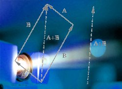
Looking at the above illustration, in which an observer, when faced with two parallel, waves as shown, as one would expects, observes them. Due to the simple effect of perspective, the wave further away appears smaller than the one closer, so what the observer observes is pretty much the same as what one sees with the Φ function.

The following diagram shows the areas of whiteness that the observer sees enclosed by red lines, while the areas of black shown by some pink ones cut off.

Now, let.s look in a bit more detail at what he sees in a more general case.

Given that the waves are not in phase, so that the area of most whiteness doesn’t occur straight in front of the observer.

The interference betweeen the two waves at a maximum at Θ=Θ₁ and Θ=-Θ₁ and at an infinite number of other greater angles (because it is equivalent to the %Phi; function, white patches occur periodically).

Notice the aquamarine line parallel to the red line on the left; this also shows a line of maximum whiteness. Lines parallel to this one will always represent an area of maximum whiteness, because it they are the lines that join areas of one wave to an identical area of the other. Even if a line intersects an area in which there is nothing but blackness, this is still an area of maximum whiteness as the nearest white areas will have as much overlap as they can.

If the observer moves parallel to the plates, then the previous line that represented the angle of maximum interference (and therefore brightness) no longer intersects the observer so one must choose a line of sight that does.

Now it should be obvious that all the lines which represent the areas of maximum whiteness will all be parallel to the lines which did so when it was in it’s original position. Therefore the observed Φ function does not change at all with parallel transformation of the observer.

Now, should the observer move perpendicular to the waves, one can similarly keep the same relative lines which represent maximum whiteness, because they’ll be parallel to the original ones and therefore totally valid.

Therefore, the observed Φ function does not change with perpendicular transformations of the observer.

Therefore, the observed Φ function is constant regardless of the position of the observer.

Solution to the grating problem

Now, what happens if the Ψ function is 2-dimensional?

Well, that depends on its symmetries. Let.s have a look at some examples:

Now wherever a point of maximum whiteness is, there’s also another one along one of the lines of symmetry (the pattern formed along the lines of symmetry because of parallel overlap is pretty much the same as the Φ function). One of the three symmetry flows from the above pattern is shown below:

Now, look at the diagram below, with an area of maximum whiteness represented by the red dot.

Now from this point we can draw three lines of symmetry:

And lets just say for simplicity that the pattern repeats ever 2 spaces. Following the horizontal line we can find some other white spaces..

and similarly we can follow the other lines around to generate the others (I.ve zoomed out a bit and haven.t depicted the underlying pattern.but that doesn.t matter much anyway)

But from each of these white patches additional lines of symmetry can be formed so that you end up with the following:

see!!!! The apparent pattern mirrors the underlying pattern structure :) (though it’s not an exact duplicate naturally). The spaces in between are blacker because less interference occurs in those. (the exact pattern isn.t really that important and can be worked out for simple patterns pretty easily but I might as well stick to the general case)

Because of what I said in section 3 this image always stays in the same position relative to you, so if you move towards it the pattern gets smaller relative to it’s surroundings but it takes up the same amount of what we see, and also the symmetry of the intereference pattern is the direct intersection of the symmetries of the underlying patterns.

Anyway that’s about it, hope it explains the interference patterns formed by wire fences and perforated screens :)

Problem

Given a circular table, place one small ball in the centre of the table and another ball of equal radius to the first at a random position. If the centre ball is hit in a random direction, what is the chance that it will hit the other ball (once it reaches the edge of the table it falls off)?

Solution

Part 1

Call the radius length of the balls r, and call the radius of the table R.

Given that the randomly placed ball is at a distance x from the centre, what’s the chance that it will be hit by the other ball? The other ball will hit it if the minimal distance between that ball and the path of the other ball is less than 2r.

But from the diagram below d = x sin θ.

So

But this only accounts for θ on one side, and so because either side of the ball can be hit either side, the total number of radians in which the colliding ball can be launched is .

And so the probability that the ball will take one of these angles as opposed to any other is

Part 2

Let P(p<x) denote the chance of a point placed at random of a disk of radius
R will be found within a distance x of the centre of the circle.

Obviously

And a simple approximation of the probability can be given in terms of the ratio of areas:

However, if there is a ball of radius r placed in the centre of the disk, the other ball will not be able to have a centre closer than 2r to the centre, so we must adjust the probability, first by truncating the probabilities below 2r, then by scaling the remaining ones so that they add up to 1.

So let , and
let’s try and calculate k and c:

Which gives the probability

Part 3

To combine the two above probabilities, we find the probability that a point will lie on between two different radii, x and x+Δx.

Getting the limit to find the probability that the point will lie on a certain radius (as a differential of course).

Now, the chance that a ball will be found on a given radius times the chance that a ball will hit is given by the multiple of the above formula by the formula in part 1.

Integrate this over the radii where the centre of the second ball can be found to get the probability that the centre ball will hit the other ball.

This is the probability that on a given table of radius R, that the ball launched from the centre will hit another randomly placed ball (both of radius r).

Of course, no generality will be lost if instead of R and r we use their ratio (The probabilities do not change. If any proof is needed of this the following substitution should suffice)

Letting , we get the probability as being

And, when graphing the ratio (x-axis) against the probability (y-axis), you get the following distribution (courtesy of gnuplot):

With the limit as the ratio approaches 2 being 0.5 (by l’Hopital’s rule).

(I thought I had this all wrong until I realized that 1/2 in gnuplot is thought of as integral division and evaluated as 0, and so until I entered 0.5 a few minutes ago in desperation as the square root power I had a seriously fucked up graph, and was about to give up hope of ever figuring out Newtonian calculus).

And another graph just for the heck of it:

Ok, enough of gnuplot for me, I’m off to buy a super-expensive graphing calculator that knows only of real numbers (unnoticed integral division, I spit on your corpse! Hah!).

A prelude

It took me a long long time to cop on to what the deal was with resolutions. But, I was, a bit ago, walking somewhere, and I saw something, or thought of something (I can’t remember what), and was like “oh, that’s just like a projective resolution”. I also had a dream about the Hilbert Syzygy theorem a few weeks ago. Can’t remember the details of that either, surely they were fascinating, though. I should probably take more descriptive notes. Ho hum… .

A difference in usage

Here’s a simple word which has markedly different connotations to mathematicians and non-mathematicians (in that the technical sense of the word can be, roughly, applied to the same situations as the non-technical one).

If you, as a nonmathematics-exposed person, say that Anne tends to project her misery onto everyone else, you would probably mean that she goes around believing everyone else to be exactly as miserable as she is.

However, to a mathematician, projection has a different intuitive feeling – projecting A onto B connotes the action of “picking out” what elements of A are common to B. That is, if you said to me that Anne tends to project her misery onto everyone else, I would be likely to feel that she only sees in other people is misery – and not only any misery, but a misery that resonantes with her own, if any. So, if I project my happiness onto you as a mathematician, I see in you what aspects of your happiness are similar to mine.

(this came out of a chat with greg).

A geometric fantasy

I was walking down the street about two weeks ago, and I thought “what if I think about myself as living in projective space?”. And I tried. Projective space is a “compactification” of our normal “affine” space, and corresponds to adding some points and calling them “infinity” (in some strikingly pleasant way), without really changing much of their local structure. But the thing is it turns spaces infinite in extent, like our “affine” space, and turns them into objects that are finite in extent (it turns the infinite line into a circle, for example). But yes, it made things feel different. The sky was no longer so far away, and everything felt as if brightly illuminated and indoors – intimate, being an appropriate word, perhaps.